The Virtual Smart Office is a simulated environment to showcase Internet of Things principals and technologies.
The simulator is built using microservice architecture running on Docker, through a docker-compose stack. The stack offers a one-stop-shop to deliver a series of microservices that demonstrate a range of IoT technologies, including:
- MQTT
- Timeseries Databases
- Real-time data capture
- AI
- Cloud
- Microservices
- Front-end visualisation
- APIs and RESTful services
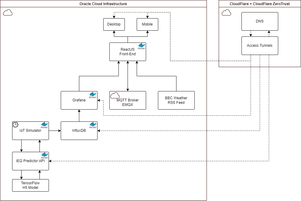
The following diagram shows the architecture of the Virtual Smart Office:
Client Application
The purpose of the client application is to provide a dashboard and ‘front-end’ to the Virtual Smart Office. The front-end of the application is developed using ReactJS with TypeScript and is deployed using Docker and docker-compose. The docker-compose file is configured to build the application using the following command:
version: "3"

services:
  client:
    container_name: virtual-smart-office-client
    hostname: virtual-smart-office-client.local
    build: ./client/
    restart: unless-stopped
    ports:
      - 40153:3000
    networks:
      - virtual-smart-office
    environment:
      - REACT_APP_MOBILE=false
      - REACT_APP_MQTT_HOST=${MQTT_HOST}
      - REACT_APP_MQTT_PORT=${MQTT_PORT}
      - REACT_APP_MQTT_USER=${MQTT_USERNAME}
      - REACT_APP_MQTT_PASSWORD=${MQTT_PASSWORD}
  controller:
    container_name: virtual-smart-office-controller
    hostname: virtual-smart-office-controller.local
    build: ./client/
    restart: unless-stopped
    ports:
      - 40154:3000
    networks:
      - virtual-smart-office
    environment:
      - REACT_APP_MOBILE=true
      - REACT_APP_MQTT_HOST=${MQTT_HOST}
      - REACT_APP_MQTT_PORT=${MQTT_PORT}
      - REACT_APP_MQTT_USER=${MQTT_USERNAME}
      - REACT_APP_MQTT_PASSWORD=${MQTT_PASSWORD}
  mosquitto:
    container_name: mqtt
    image: eclipse-mosquitto
    restart: always
    networks:
      virtual-smart-office:
        ipv4_address: 172.20.0.4
    volumes:
      - ./data/mqtt/config:/mosquitto/config
      - ./data/mqtt/data:/mosquitto/data
      - ./data/mqtt/log:/mosquitto/log
    ports:
      - 40155:9001
networks:
  virtual-smart-office:
    driver: bridge
    ipam:
      config:
        - subnet: 172.20.0.0/24
The docker-compose file builds two instances of the client application, one for the main application and one for the mobile application. The main application is accessible via the following URL: https://iot-sim.grahamcoulby.co.uk/. The mobile application is accessible via the following URL: https://iot-sim-controller.grahamcoulby.co.uk/.
The Dockerfile for the React application is as follows:
FROM node:16.14.0-alpine

WORKDIR /app

# add `/app/node_modules/.bin` to $PATH
ENV PATH /app/node_modules/.bin:$PATH


# install app dependencies
COPY package.json ./
# COPY package-lock.json ./
RUN npm install
RUN npm install [email protected] -g

# add app
COPY . ./

# start app
CMD ["npm", "start"]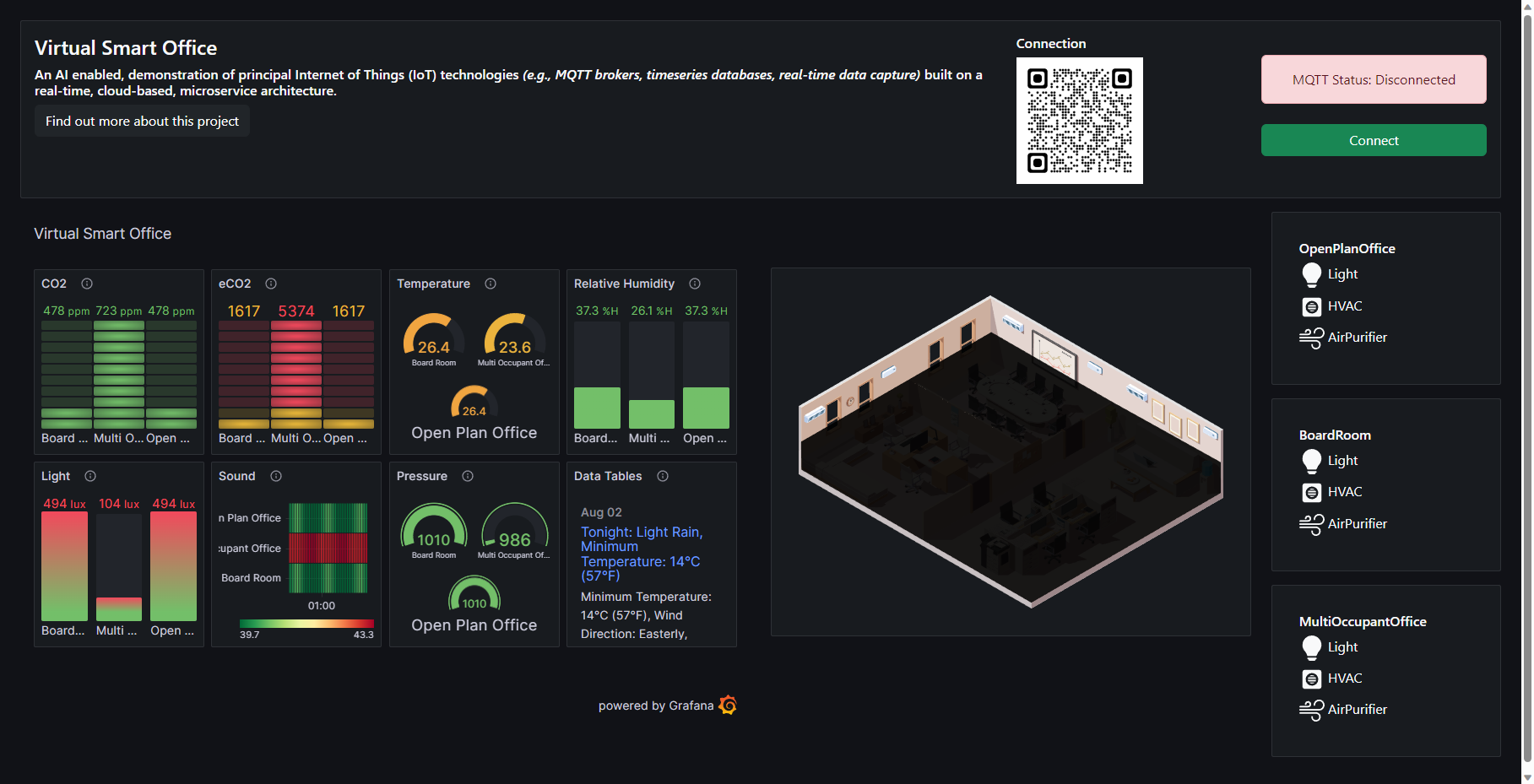
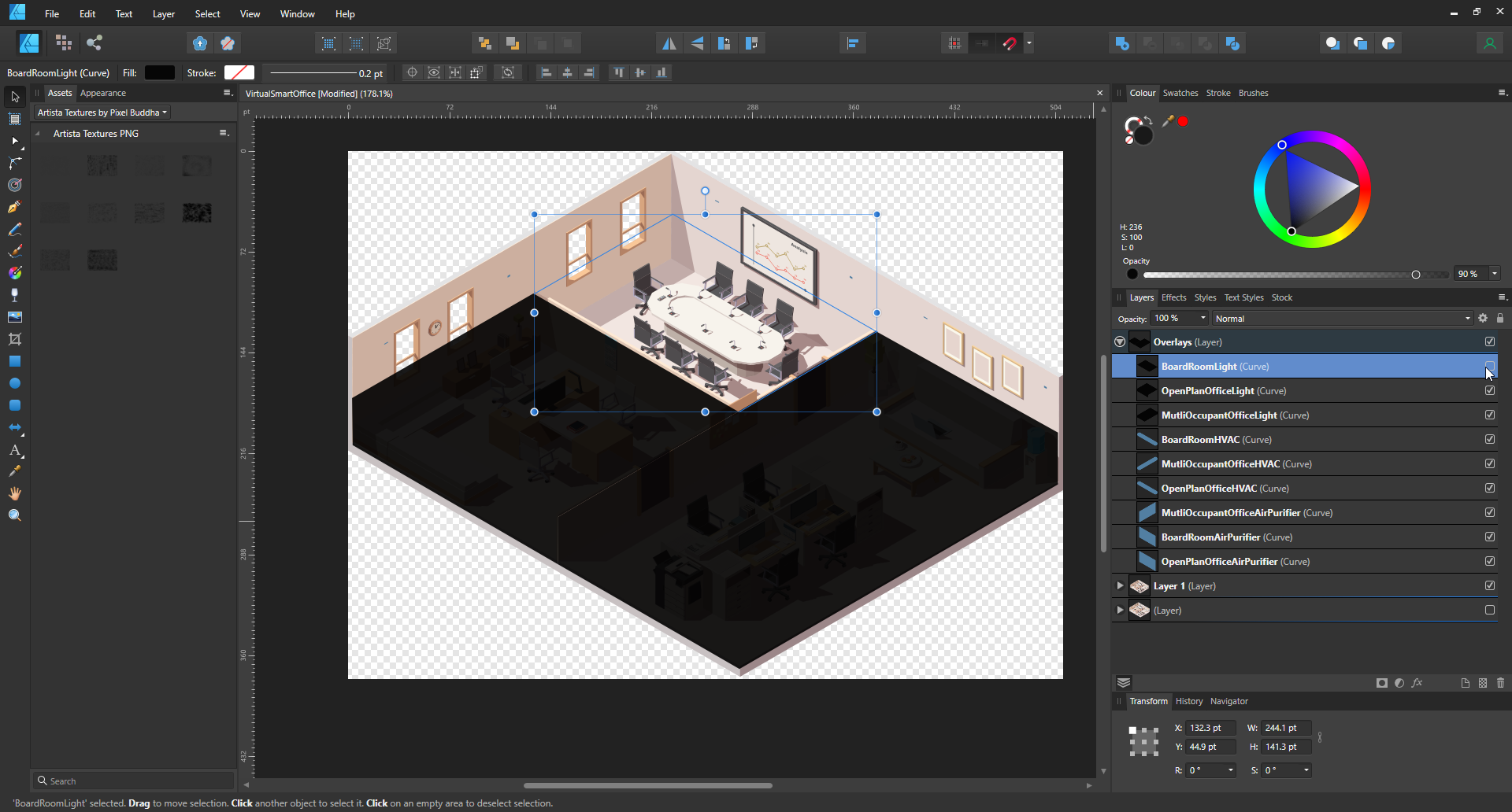
SVG Model
The application provides a graphical SVG model, which I got from FreePik during my Ph.D. I modified the SVG using Affinity Designer and added interactive elements that can be ‘turned on’ and ‘turned off’. These elements are:
- Air Conditioners
- Air Purifiers
- Lights
The state of these elements is controlled by MQTT messages, which are published and subscribed to by the client application. The client application also publishes MQTT messages to control the state of these elements.
MQTT Controls
The client also displays a series of toggle switches. These provide a real-time, multi-pub/sub interface, whereby multiple clients can publish and subscribe to the MQTT messages being transmitted/received from/to the client.
The virtual Air Conditioners and Air Purifiers used in this simulation do not have an effect on the data generated in the graphs. Their only purpose is to simulate/showcase MQTT control over the building.
Data Graphs
The application also displays sensor telemetry from simulated IoT environmental quality sensors. The data from these ‘devices’ are generated by the IEQ Simulator service, which is explained below. The graph dashboard is embedded into this application and is generated using Grafana, which takes a data feed from InfluxDB.
Weather RSS
The application also displays a weather RSS feed, which is pulled from BBC Weather. This is just to simulate fetching data from an external source.
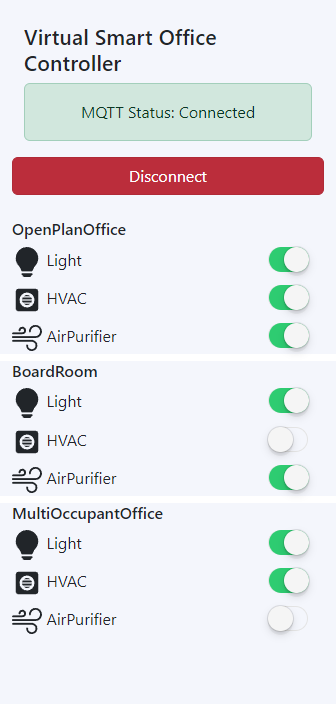
Mobile Application
There is a mobile application as well, which is accessible via the QR code on the client application (https://iot-sim-controller.grahamcoulby.co.uk/). The mobile application is actually the same React application, but with a different UI. The docker-compose file uses the same build command as the client application:
build: ./client/However, the mobile application sets the following flag in the environment variables:
REACT_APP_MOBILE=trueWhen the React app sees this flag, it shows only the toggle switches and the connect buttons, this saved writing two separate implementations of the application - but also allows the main application to be scalable to different screen sizes - without limiting the functionality of the application.
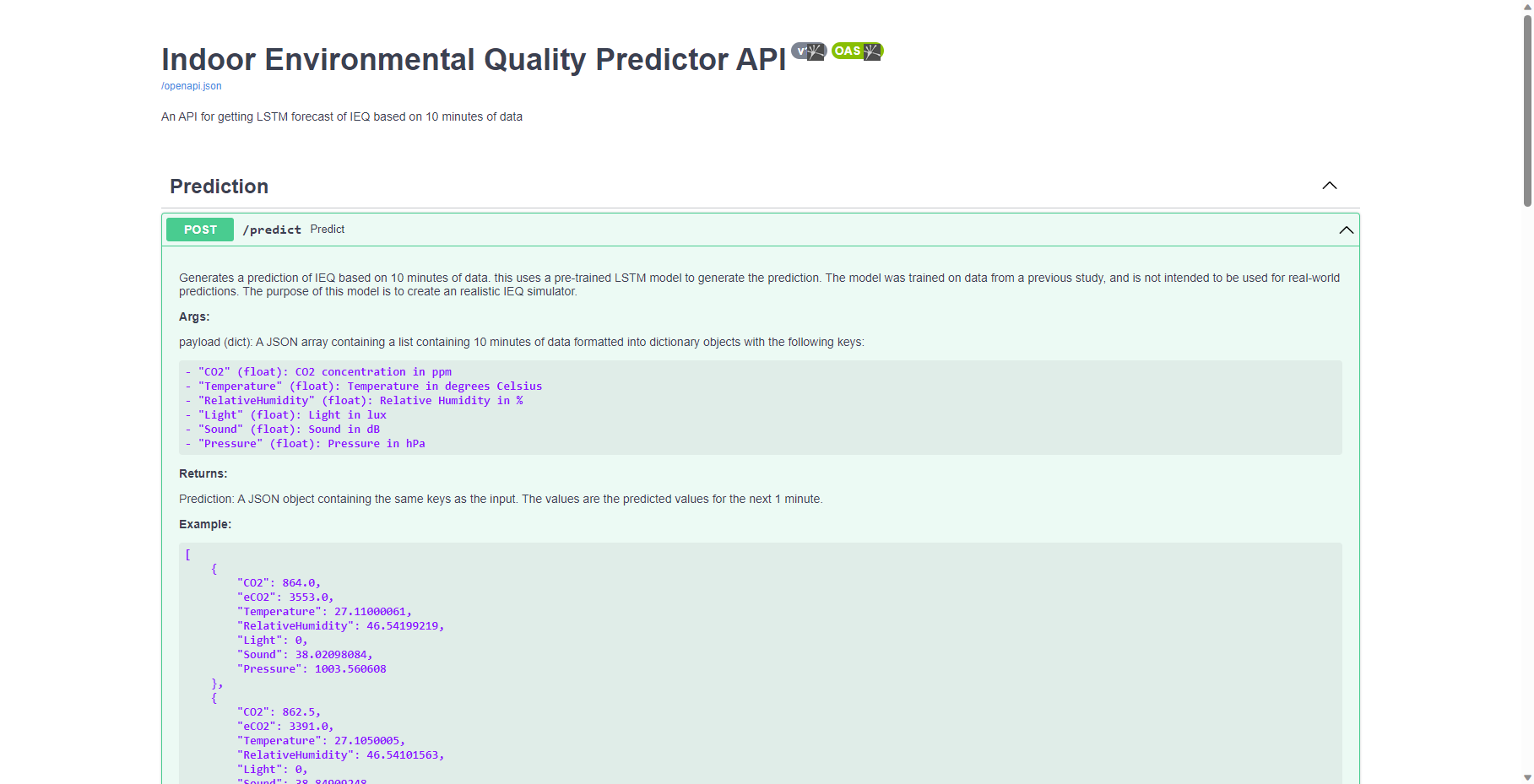
IEQ Predictor API
An IEQ predictor API was created to generate realistic 'fake' sensor data. The API was developed using the python FastAPI framework.
The Dockerfile for the API is as follows:
FROM python:3.10-slim

RUN apt-get update
RUN apt-get install -y gcc
RUN apt-get install -y default-libmysqlclient-dev
ENV PYTHONBUFFERED 1

COPY . /app
COPY ./requirements.txt /app

WORKDIR /app

RUN pip3 install -r requirements.txt

EXPOSE 8000

CMD ["uvicorn", "main:app", "--host=0.0.0.0", "--port=8000", "--reload"]
The data are generated using an Autoregressive Long Short Term Memory Neural Network, which is trained on IEQ data captured from a previous study entitled “Personalised and Sustainable IEQ Monitoring: Use of Multi-Modal and Pervasive Technologies” (https://doi.org/10.3390/ijerph20064897). The data were captured from a series of sensors placed in a physical study location. The data were captured over a period of 6 months, and the data were captured at 1-minute intervals. Data were captured from the following sensors:
- CO2 Sensor
- eCO2 Sensor
- Temperature Sensor
- Humidity Sensor
- Light Sensor
- Sound Sensor
- Pressure Sensor
The LSTM model was trained to generate a new sensor reading for each of the sensors based on the previous 10 readings. The model was trained on 70% of the data, and the remaining 30% was used to validated and test the model. The model was trained using the Keras library, and the model was saved as a .h5 file. The model was then integrated into a FastAPI application, which provides data to the IEQ Simulator service. The documentation for the API can be found here: https://ieq-predict.grahamcoulby.co.uk/docs
IoT Simulator Service
The IoT Simulator service is a python application that generates simulated data from a series of IoT devices. The application calls the IEQ Predictor API to generate the data for the sensors. Since the IEQ Predictor service requires the previous 10 readings to generate a new reading, the IoT Simulator service creates the payload for the API by taking a sample from the original dataset used to train the model.
To create the data the following method is used:
def build_df(room, dayOffset=0):
    """Builds the df from the ImputationResult.csv file. This file contains
    the imputed data from a previous study (https://doi.org/10.3390/ijerph20064897)
    and is used to train the model. The df is built by reading the CSV file
    and adjusting the timestamps to the current time. This is done by finding the
    last record in the df with the same day, hour and minute as the current
    timestamp. The df is then sliced from the start to the index of the last
    record. The date is then shifted by the number of days between the last record
    and the current timestamp. This creates a df that is simulating the current
    historical data.
    """
    global dfs
    # Read in the CSV data
    df = pd.read_csv(f"{BASE_PATH}/ImputationResult.csv")

    df["dt"] = pd.to_datetime(df.pop("dt"), format="%Y-%m-%d %H:%M:%S")

    # Get current time
    now = datetime.now(pytz.timezone("Europe/London"))
    hour = now.hour
    minute = now.minute
    weekday = now.weekday() + 1 - dayOffset
    if weekday <= 0:
        weekday = 7
    elif weekday > 7:
        weekday = 1

    # Get the last index from the df where the Day, Hour and Minute
    # match the current timestamp
    idx = np.where(
        df["DayNumber"].eq(weekday) & df["Hour"].eq(hour) & df["Minute"].eq(minute + 1)
    )[0][-1]

    # Set the dateframe to a slice from start to the previously found index
    df = df[:idx]

    # find the datetime in the lastrow and use it to find the number of days
    # that have passed between that datapoint and the current timestamp
    lastRow = df.iloc[-1]
    oldDateStr = f"{lastRow['dt']} {lastRow['Hour']}:{lastRow['Minute']}"
    oldTimestamp = parse(oldDateStr)

    # store the number of days to offset for later
    dayOffset = (datetime.now() - oldTimestamp).days

    # Shift the date by the dayOffset
    df["shifted_dt"] = df.dt + pd.Timedelta(days=dayOffset)

    # Convert the shifted_dt to a datetime dataframe
    date_time = pd.to_datetime(df["shifted_dt"], format="%Y-%M-%D %H:%M:%S")

    dayInMins = 24 * 60

    timestamp_s = date_time.map(pd.Timestamp.timestamp)
    df["timestamp_s"] = timestamp_s
    df["Day sin"] = np.sin(timestamp_s * (2 * np.pi / dayInMins))
    df["Day cos"] = np.cos(timestamp_s * (2 * np.pi / dayInMins))

    # Filter the df to only include the columns we need for the model
    dfs[room] = df[LABELS].tail(10)
Essentially this method takes the original dataset, and finds the last record that matches the current day, hour and minute. It then slices the dataset from the start to the index of the last record. The date is then shifted by the number of days between the last record and the current timestamp. This creates a df that is simulating the current historical data. The df is later converted to a numpy array and is then passed to the IEQ Predictor API, which generates a new reading for each of the sensors. The data is then published to InfluxDB, which is then visualised in Grafana. This approach also ensures that the data being used in production is realistic, and is based on real data, but is not the same data that was used to train the model. The actual sample that is selected comes from the test/validation dataset, which was not used to train the model. This prevents the model from just returning the same data that was used to train it.
The Dockerfile for the IoT Simulator service can be found here:
FROM python:3.11.4-slim
COPY main.py ./
COPY models.py ./
COPY ImputationResult.csv ./
COPY requirements.txt ./
COPY .env ./
RUN /usr/local/bin/python -m pip install --upgrade pip && pip3 install -r requirements.txt
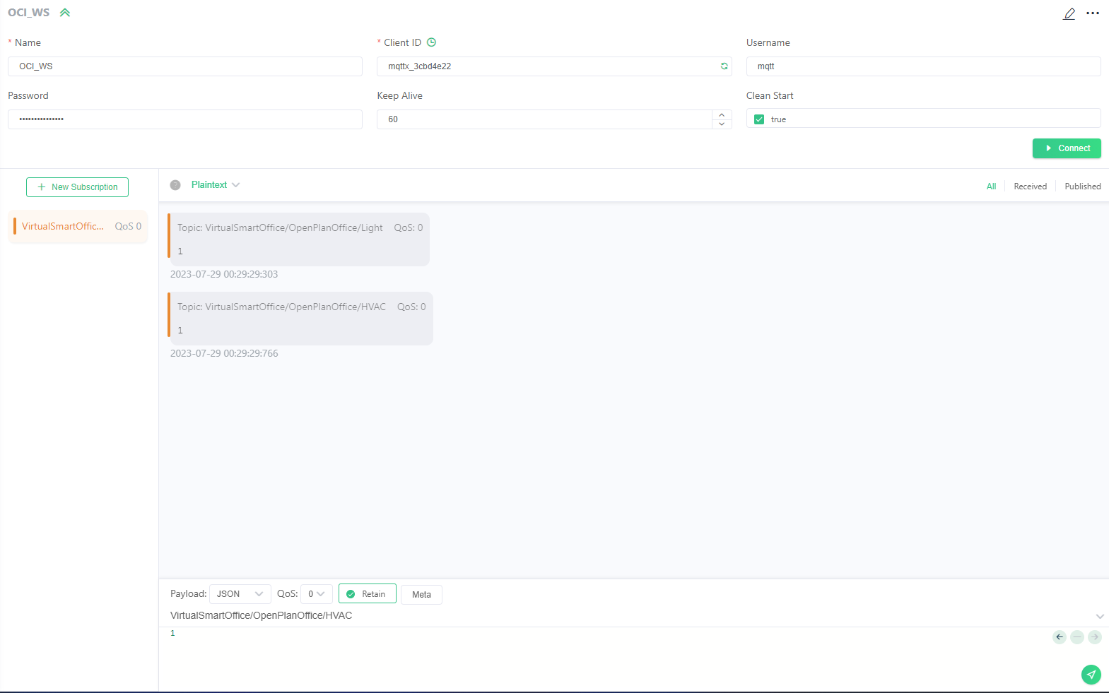
CMD ["python", "main.py"]MQTT
I had originally developed (and actually have) a working stack that uses a local Mosquitto MQTT broker. However, since the client application is hosted behind an SSL certificate, due to secure CloudFlare tunnels, I was unable to connect to the local broker. I had tried to use a reverse proxy to connect to the local broker, but this was conflicting with the CloudFlare tunnels I setup for this application. I then decided to use a public MQTT broker for the purposes of testing, which would allow me to connect to the broker from via a secure websocker from the client application. I used the EMQX broker, which is a public broker that allows you to create a free account. The client application connects to the broker using the Paho MQTT library, and the client subscribes to the following topics:
| ParentTopic | Room | Sensor | Topic |
|---|---|---|---|
| VirtualSmartOffice | BoardRoom | CO2 | VirtualSmartOffice/BoardRoom/CO2 |
| VirtualSmartOffice | BoardRoom | eCO2 | VirtualSmartOffice/BoardRoom/eCO2 |
| VirtualSmartOffice | BoardRoom | Temperature | VirtualSmartOffice/BoardRoom/Temperature |
| VirtualSmartOffice | BoardRoom | Humidity | VirtualSmartOffice/BoardRoom/Humidity |
| VirtualSmartOffice | BoardRoom | Light | VirtualSmartOffice/BoardRoom/Light |
| VirtualSmartOffice | BoardRoom | Sound | VirtualSmartOffice/BoardRoom/Sound |
| VirtualSmartOffice | BoardRoom | Pressure | VirtualSmartOffice/BoardRoom/Pressure |
| VirtualSmartOffice | OpenPlanOffice | CO2 | VirtualSmartOffice/OpenPlanOffice/CO2 |
| VirtualSmartOffice | OpenPlanOffice | eCO2 | VirtualSmartOffice/OpenPlanOffice/eCO2 |
| VirtualSmartOffice | OpenPlanOffice | Temperature | VirtualSmartOffice/OpenPlanOffice/Temperature |
| VirtualSmartOffice | OpenPlanOffice | Humidity | VirtualSmartOffice/OpenPlanOffice/Humidity |
| VirtualSmartOffice | OpenPlanOffice | Light | VirtualSmartOffice/OpenPlanOffice/Light |
| VirtualSmartOffice | OpenPlanOffice | Sound | VirtualSmartOffice/OpenPlanOffice/Sound |
| VirtualSmartOffice | OpenPlanOffice | Pressure | VirtualSmartOffice/OpenPlanOffice/Pressure |
| VirtualSmartOffice | MultiOccupantOffice | CO2 | VirtualSmartOffice/MultiOccupantOffice/CO2 |
| VirtualSmartOffice | MultiOccupantOffice | eCO2 | VirtualSmartOffice/MultiOccupantOffice/eCO2 |
| VirtualSmartOffice | MultiOccupantOffice | Temperature | VirtualSmartOffice/MultiOccupantOffice/Temperature |
| VirtualSmartOffice | MultiOccupantOffice | Humidity | VirtualSmartOffice/MultiOccupantOffice/Humidity |
| VirtualSmartOffice | MultiOccupantOffice | Light | VirtualSmartOffice/MultiOccupantOffice/Light |
| VirtualSmartOffice | MultiOccupantOffice | Sound | VirtualSmartOffice/MultiOccupantOffice/Sound |
| VirtualSmartOffice | MultiOccupantOffice | Pressure | VirtualSmartOffice/MultiOccupantOffice/Pressure |
Timeseries Database (InfluxDB)
I chose to use InfluxDB because it is a time series database, which is ideal for storing the sensor data. The data is stored in the following format:
| Time | Room | Sensor | Value |
|---|---|---|---|
| 2021-05-01T00:00:00Z | BoardRoom | CO2 | 400 |
| 2021-05-01T00:00:00Z | BoardRoom | eCO2 | 400 |
| 2021-05-01T00:00:00Z | BoardRoom | Temperature | 20 |
the data is then visualised in Grafana. Timeseries databases are ideal for storing data that is generated over time, and is often used for IoT applications. InfluxDB is also very easy to setup and use, and has a very good integration with Grafana.
The docker-compose file for the InfluxDB service can be found here:
version: "3"

networks:
  metrics:
    external: false

services:
  influxdb:
    image: influxdb:latest
    container_name: influxdb
    restart: always
    networks: [metrics]
    ports:
      - "8086:8086"
    volumes:
      - $HOME/docker/influxdb/data:/var/lib/influxdb
      - $HOME/docker/influxdb/influxdb.conf:/etc/influxdb/influxdb.conf:ro
      - $HOME/docker/influxdb/init:/docker-entrypoint-initdb.d
    environment:
      - INFLUXDB_ADMIN_USER=${INFLUXDB_USERNAME} # sourced from .env
      - INFLUXDB_ADMIN_PASSWORD=${INFLUXDB_PASSWORD} # sourced from .env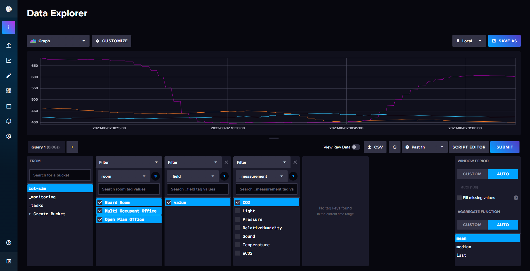
Data Visualisations (Grafana)
Grafana was chosen because its has a very good integration with InfluxDB, and it is very easy to setup and use. Grafana is a data visualisation tool that allows you to create dashboards that can be used to visualise data from a variety of sources. Grafana is also very easy to setup and use, and has a very good integration with InfluxDB. The dashboards can be made public, which allows them to be embedded into external applications with ease... So long as the following environment variables are setup when the container is created:
- GF_SECURITY_ALLOW_EMBEDDING=true
- GF_FEATURE_TOGGLES_ENABLE=publicDashboards
The full docker-compose file for the Grafana service can be found here:
services:
  grafana:
    image: grafana/grafana:latest
    container_name: grafana
    security_opt:
      - no-new-privileges:true
    restart: unless-stopped
    networks:
      - default
    ports:
      - "7564:3000"
    # volumes:
    #   - ./data/grafana-storage:/var/lib/grafana:Z
    #   - ./data/grafana-provisioning:/etc/grafana/provisioning:Z
    environment:
      - GF_SECURITY_ADMIN_USER=${GRAFANA_USERNAME}
      - GF_SECURITY_ADMIN_PASSWORD=${GRAFANA_PASSWORD}
      - GF_SECURITY_ALLOW_EMBEDDING=true
      - GF_FEATURE_TOGGLES_ENABLE=publicDashboards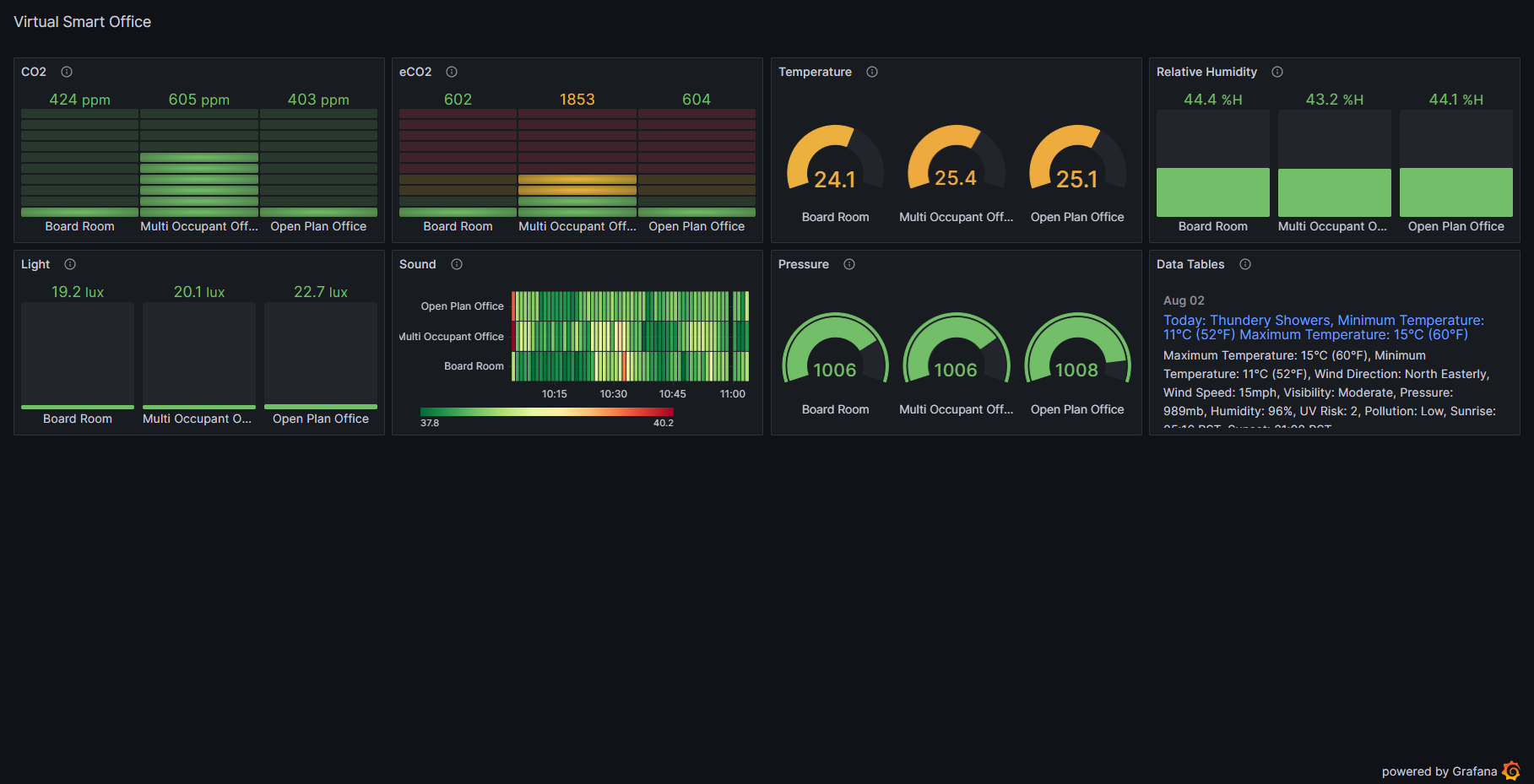
Docker and Docker Compose
Each service within this stack is containerised using Docker and brought online using docker-compose. Wherever possible I try to use Docker Compose over vanilla Docker because it is much easier to manage multiple containers using a single docker-compose.yml file and the files are both easier to understand and give you a persistent record of the configuration of the stack.
CloudFlare
I migrated to CloudFlare as my domain provide about a year ago as I was using the service for caching and traffic monitoring. For this project I setup tunnels to provide DNS records for services running on Oracle Cloud Infrastructure. I also used CloudFlare to generate the SSL certificates for those services.
Oracle Cloud Infrastructure
I used Oracle Cloud Infrastructure to host all of the services in this stack. I chose to use Oracle Cloud Infrastructure because I was able to get a free ARM instance with 24GB of RAM and 4 vCPUs. Previously I have used this just for testing docker images, but I found that it was more than capable of running the entire stack, with plenty of room to spare. I was keen to use a cloud provider for this project as not only did I want it to be accessible from anywhere, I wanted the project to be realistic to typical IoT deployments, which would typically be hosted in the cloud.
API
I intend to develop a second FastAPI service, which will be used to provide an API for the InfluxDB database. This will provide a persistent API for capturing simulated sensor data for testing and development purposes. This will be developed in a separate repository.